NONDESTRUCTIVE TESTING HANDBOOK -
Electromagnetic Testing
Manual de Ensaio Não Destrutivo - Ensaio Eletromagnético
- Parte 1. Introdução aos Instrumentos do Ensaio de Correntes Parasitas
- Funções
- Propósito
- Especificações Críticas
- Apresentação dos Dados de Correntes Parasitas
- Parte 2. Funções dos Sistemas de Correntes Parasitas
- Excitação
- Modulação
- Multiplexação
- Configuração da Excitação
- Parte 3. Demodulação
- Preparação
- Demodulação e Análise
- Parte 4. Saída
- Mostrador
- Filtragem
- Reconhecimento de Sinais
- Controle
1 INTRODUÇÃO AOS INTRUMENTOS DO ENSAIO DE CORRENTES PARASITAS
Four techniques of electromagnetic testing
are well developed and used for
commercial applications: alternating
current field measurement, eddy current
testing, magnetic flux leakage testing and
remote field testing. Each of these four
electromagnetic techniques has specific
application areas where it has shown
some advantage over the other three as
well as other nondestructive test methods.
All four share core instrumentation
concepts and many of the following
details are applicable to all four
techniques. A general purpose eddy
current instrument can be adapted to
perform any of these tests.
in addition to these four techniques,
several additional electromagnetic test
processes provide some test capabilities
but are less developed. This chapter
focuses specifically on instrumentation for
the eddy current technique.
1.1 FUNÇÕES
1.1.1 PROPÓSITO
The purpose of an eddy current
instrument is to drive an eddy current
transducer, or probe, with an excitation
signal and to analyze the signal
modulated by that transducer for
information pertinent to the application.
Applications for eddy current
instrumentation vary from use on a
manufacturing floor for verification of
whethera part has been heat treated to
evaluation of nuclear steam generator
tubing.
Test frequencies may range from a few
hertz for testing ferromagnetic parts to
megahertz for testing thin titanium. The
instrument may use a fixed frequency for
testing a single property, as does a simple
conductivity meter, or it may use multiple
frequencies for discrimination of multiple
conditions when analyzing heat treated
materials or heat exchanger tubing.
A wide variety of instrumentation
exists today. Single-frequency units with
an analog meter allow an operator to
distinguish discontinuities by needle
position. Other single-frequency units use
a bar graph to display a single parameter
and trigger an alarm to allowa controller
to properly dispose of a bad part.
Complex, general purpose instruments
may be used in multifrequency tests of up
to 32 frequencies over six orders of
magnitude, from 10 Hz to 10 MHz. These
instruments range from handheld and
desktop units to remote data acquisition
systems on networks of dedicated
workstations that also control robotics
and run sophisticated data analysis
programs.
1.1.2 ESPECIFICAÇÕES CRÍTICAS
Several specifications critical to an eddy
current test must be carefully considered
by the instrumentation designer.
Frequency Accuracy.
The frequency is
absolutely critical because it determines
eddy current depth of penetration and the
amplitude and phase of a discontinuity
response. Distortion of the applied
waveform should be minimized and
quantified because distortion is caused by
other frequency components in the
signal.
Drive Accuracy.
The amplitude of the
drive determines the amplitude of the
response. It should be well controlled and
its frequency response should be specified.
Gain Linearity and Accuracy.
The
amplitude and phase characteristics of all
gain stages must be qualified for
adherence to a standard or specification
appropriate to the application, especially
so that adjustment of variable gain stages
does not distort a signal.
Horizontal and Vertical Deviation.
Gain of
the in-phase and out-of-phase
components of a signal must be
controlled to prevent unwanted distortion
of a signal. A flattened appearance caused
by unequal gains is a liability for some
applications but is very useful in others.
In a typical heat exchanger test, a
flattened appearance would cause
misrepresentation of the data whereas, in
the rotating test of a rivet hole for surface
breaking cracks, it can be used to
minimize liftoff noise and accentuate a
crack signal.
Quadrature Accuracy.
The phase of
reference signals must be well controlled
and the response of the display must be
designed to ensure that the in-phase and
out-of-phase components are truly at
90 degrees electrically and that they are
displayed orthogonally.
Digitization Rate.
The digitization rate for
a digital system is the number of samples
per unit of transducer travel. This rate is
critical for determining the response to a
discontinuity. Too few samples over the
length of the test object may cause a
discontinuity to be missed altogether or at
least to be highly distorted. Digitization
rate must be determined from the
application criteria. If detection is the
only requirement, a lower digitization rate
may be sufficient to produce a signal that
breaks the desired alarm level. If analysis
of the signal is required, the digitization
rate must be high enough that an
accurate picture of the discontinuity
signal is presented without distortion.
Sample Rate.
The sample rate for a digital
system is the number of interrogations per
unit of time, often given as samples per
second. To calculate the required sample
rate for a test, the transducer speed is
multiplied by the desired digitization rate.
Because the sample rate is the
determining factor for the digitization
rate, it must be high enough to permit the
required transducer speed and must be
accurate so that the digitization of signals
is evenly spaced along the surface of the
test object(s).
Some instruments have an external
sample trigger that may be activated by
an encoder system measuring actual
distance traveled. This trigger ensures an
accurate digitization rate for varying
transducer speed as long as the maximum
sample rate of the instrument is not
exceeded.
Bandwidth.
Bandwidth is not to be
confused with sample rate. Rather than
the number of samples taken, bandwidth
governs the response of the system as a
function of frequency and is measured in
hertz. It is usually determined by
demodulator and filter characteristics.
Exceeding the bandwidth of the
instrument will cause signals to be
attenuated and distorted because some of
their frequency components will be
filtered out. Although distortion may be
acceptable in situations where
detectability can be demonstrated, as with
known types of discontinuities on a high
speed manufacturing line, distortion may
prevent detection of discontinuities or
adversely affect the ability to characterize
them. A variable frequency, external
modulator is often used to measure and
characterize bandwidth through all stages
of an instrument.
Stability.
System stability and response to
temperature and aging variations must be
demonstrated to ensure that excessive
drift does not occur between calibration
intervals. This is especially important in
the manufacturing world where a very
small alarm may be placed around a
baseline signal and the equipment run
continuously for months or even years at
a time.
Two factors govern the design of any
test instrumentation: (1) signal-to-noise
ratio and (2) dynamic range. These factors
are linked to one another and, in the
design of an instrument, care must be
taken to maximize the signal-to-noise
ratio and to allow adequate dynamic
range for signals of interest.
Ultimately, the goal of a nondestructive
test is to produce a discontinuity signal
distinguishable from surrounding noise
and to view a desired range of signals
without distortion.
Dynamic range can be defined as the
ratio of the total signal range of an
instrument divided by the amplitude of
the noise signal. This range can be
expressed either as a ratio or as decibels or
bits in a digital system. For example, a
16-bit analog-to-digital converter with a
+10 V input may have one bit (305 pV) of
noise. This noise level yields a dynamic
range of 15 bits (range of 16:1 noise bit),
65 574:1 (20 V to 305 pV) or 96 GB.
If the minimally acceptable
signal-to-noise ratio for a test is 3:1, then
the dynamic range available for signals is
the total range divided by the minimum
signal or is the total range divided by
three times the noise.
Noise is a very general term and can be
defined as any unwanted signal affecting
the test. Common sources of noise in
electromagnetic testing are the following:
(1) electronic noise inherent to the
instrumentation; (2) external
electromagnetic interference, radiated or
conducted; (3) transducer imbalance;
(4) triboelectric, or microphonic, noise in
the transducer cabling; and (5) test object
irregularities, such as wall thickness
variations in a rotating pancake coil tube
test. These all contribute to a reduction in
both signal-to-noise ratio and dynamic
range.
Each stage of the instrumentation acts
as a dynamic range window, or
bottleneck, and adds some amount of
noise toa test.
1.2 APRESENTAÇÃO DOS DADOS DE CORRENTES PARASITAS
Any eddy current or remote field system is
measuring an alternating magnetic field
as modified by a test object. The voltage
signal from the transducer may be
represented as a phasor in the complex
plane with an amplitude and phase angle
(Fig. 1). The technique used to display the
phasor depends on the application of the
test being performed.

Legenda:
A = amplitude
phi = phase
Ficure 1. Phasor in complex plane.
In the simplest instruments, the
amplitude of this phasor alone may
contain the desired information. A voltage
readout in the form of a meter or bar
graph may constitute the only display,
usually supplemented by an alarm output,
triggered when the voltage exceeds a set
level.
In most instruments, however, the
incoming signal is processed to obtain
either amplitude and phase or real and
imaginary components of the phasor. This
provides two known components per
phasor, which allows the separation of
two variables. Multiple frequencies add
additional known values for
discriminating additional variables. These
components are most commonly
displayed on an oscilloscope display,
where the resultant dot moves around the
display as the signal changes. Different
mechanisms produce characteristic
patterns of change of the signal voltage
and these patterns may be scrutinized in
detail to evaluate the object being tested.
To maximize the dynamic range and
signal-to-noise characteristics of an
instrument, various nulling (balancing)
techniques are used. These basically
subtract out the phasor of a null signal
from a transducer on a good area ofa test
object so that the resultant dot is centered
at the zero point of the display. The signal
patterns are then rotated around the zero
to show the discontinuity patterns as
desired. It is common for the operator to
choose a frequency at which the liftoff of
the transducer from the test object lies on
the horizontal axis of the display and the
desired discontinuity signal displays
vertically. Operators can then watch for
vertical indications and ignore the liftoff
signal. A
number of simple eddy current
instruments use this technique and
display only one component on a meter
or bar graph with capabilities of triggering
an alarm on signals that exceed a set
level.
A number of specialized instruments
process the phasor signal for a particular
quantity. Conductivity meters are a
typical example. The signal is processed
by algorithms that calculate the
conductivity of a specimen and display it
as a number ona digital readout. Some
conductivity meters also calculate and
provide a number for the distance of the
transducer from the specimen for
measurement of coating thickness. There
are dedicated coating thickness gages
available too.
Hugo Libby laid his groundwork
measuring the impedance of eddy current
coils with which he performed his test.!
He called the complex plane on which he
displayed data the impedance plane. The
impedance plane has become the most
common display for electromagnetic test
data, whether used with impedance
probes, reflection (driver pickup or
send/receive) probes or even display of
remote field data.
When Libby built his first eddy current
instrument, he attached the cables to the
oscilloscope to display the in-phase
component (which he called imaginary)
on the horizontal axis and the
out-of-phase component (called real) on
the vertical axis. He then rotated the field
to get the real component back onto the
horizontal axis. This rotation leaves a
phase angle of zero on the left horizontal
axis and phase angle increasing in a
clockwise direction. This is in contrast to
the true complex plane, which has a
phase angle of zero on the right
horizontal axis and phase angle increasing
in the counterclockwise direction. This
interesting artifact is often confusing for
engineers new to nondestructive testing.
In practice, most testing is done relative
to a reference standard with the field
rotated such that zero phase is defined to
be a particular indication, most often the
transducer liftoff signal.
2. FUNÇÕES DOS SISTEMAS DE CORRENTES PARASITAS
For an eddy current system to provide
information to an inspector, five
functional steps have to be performed
(Fig. 2): excitation, modulation, signal
preparation, signal demodulation and
signal display. An optional sixth step
would be test object handling equipment.

Ficure 2. Internal functions of eddy current test instrument.
2.1. EXCITAÇÃO
The excitation portion of an eddy current
instrument consists of signal generation
and amplifiers to drive the transducers.
The signal generator (or oscillator)
provides sine wave excitation for the test
coil. Single-frequency systems have one
fixed frequency whereas multifrequency
systems can apply several frequencies to
provide multiple-parameter options. The
application determines the required
frequency and the number of frequencies
to be used. Additional frequencies are
selected to provide additional test
parameters for specimens with multiple
variables. In this way, the number of
measured parameters will equal or exceed
the number of variables to allow
discrimination of all desired discontinuity
types. More complex test specimen
problems require more sophisticated
instrumentation to test the specimens
adequately.
Early systems had what were called
frequency modules, designed to generate
one frequency only. If a different
frequency was wanted, then the physical
module was replaced with another that
would operate at a different frequency.
Most modern systems have a frequency
generator that will operate over a very
wide frequency range. This means that
the operator can make the best choice of
frequencies to apply to a given
application. On analog systems, this
would be controlled through a switch. On
digital systems, it can be accomplished
through defining the digital parameters
on a menu of available options.
The signal generators themselves vary
from simple, fixed frequency, schmitt
trigger oscillators, to phase locked loops,
sine lookup tables and digital data
synthesizers. Some digital systems filter a
square wave clock to provide an
adequately clean sine wave to apply to the
transducer. The design emphasis in this
stage is to produce a signal of adequate
frequency accuracy, frequency stability
and low distortion for a reliable test. If
frequency is inaccurate, depth of
penetration is not as expected and
analysis of any resulting signal is
correspondingly inaccurate. If the
frequency is allowed to drift, results will
vary accordingly throughout the test, with
the result that good parts may be rejected
or that critical discontinuities may be
ignored — or both. Excessive distortion
on the excitation signal introduces into
the test additional frequencies that may
cause undesired signal results or may
simply reduce the signal-to-noise ratio of
the test. A certain amount of broadband
electronic noise is present on any signal.
It is important that it be minimized here
because excitation is the beginning of the
signal train through the instrument.
Many instruments also derive the
timing functions for the demodulation
stage from the oscillator. The amplitude
and frequency characteristics must be well
controlled because any inaccuracy,
frequency jitter or voltage noise on these
reference signals will be added into the
test signal in the demodulator stage. The
quadrature, the relative timing, of these
signals must be accurately controlled so
that the in-phase and out-of-phase
components of the test signals are
accurately demodulated at 90 degrees
from each other.
2.2 MODULAÇÃO
2.2.1 MULTIPLEXAÇÃO
Single-frequency testers apply one selected
frequency to the transducer. This
frequency may be permanently set as in a
60 kHz conductivity meter, which uses a
dedicated coil to discriminate liftoff and
conductivity.
Single-frequency instruments intended
for general purposes allow selection of the
frequency to fit the application and are
capable of driving a wide range of
transducers.
Multifrequency testers are normally set
up to generate from two to 32 different
frequencies selectable by the operator.
Multifrequency testing is accomplished
through three different techniques:
- (1) time domain multiplexing,
- (2) frequency domain multiplexing and
- (3) pulsed frequency testing.
Multiplexing means sending multiple
frequencies over a single channel to the
test coil. Instruments using time domain
and frequency domain multiplexing
generate and switch among a number of
discrete frequencies. Each technique has
advantages and disadvantages. Some
instruments can multiplex in the
frequency domain, in the time domain or
in both concurrently.
With time domain multiplexing,
multiple frequencies are generated
sequentially (Fig. 3). In digital systems, a
number of frequency time slots are
selected. Analog systems usually have a
fixed number of time slots. The coil is
energized at one frequency for a
predetermined period of time. The
frequency generator is then switched to a
different frequency in the second time
slot for another specific period of time.
This process continues until all selected
frequencies have been applied to the coil.
The process then starts again with
frequency number one. Timing of each
specific frequency is critical to accurately
process and display the information from
each individual time slot on the output
device.

Legenda:
A. 400 kHz.
B. 200 kHz.
C. 100 kHz.
D. 20 kHz.
Ficure 3. Time domain multiplexed
waveform.
With frequency domain multiplexing,
multiple frequencies are applied to a coil
at the same time, so this means of
multiplexing is commonly called
simultaneous injection (Fig. 4). In this
scenario, all of the selected frequencies are
applied to the coil continuously. The
recurring pattern in Fig. 4 is not caused by
sequential input of frequencies as in the
time domain multiplexing of Fig. 3.

Ficure 4. Frequency domain multiplexed
waveform, for simultaneous application of
frequencies at 400, 200, 100 and 20 kHz.
Pulsed frequency instruments apply a
unit pulse to a transducer. A unit pulse is
a short, rapidly rising and falling pulse
containing an infinite series of harmonics.
This pulse can be mathematically shown
to contain these harmonics. (Harmonics
are an infinite series of frequencies that
are multiples of the base frequency.) These
instruments usually display a time based
result and allow gating of the signal at
selectable time intervals to analyze the
data for a specific frequency. This gating is
very familiar to operators of ultrasonic
testing equipment and provides a
corollary to the time of flight of a
sound
wave.
The advantages of time domain
multiplexing are that it permits maximum
power to be applied to the transducer and
that it permits maximum use of the
dynamic range of an instrument at each
discrete frequency. Drive and gain stages
can be optimized for each time slot.
Optimizing can be very helpful for
analyzing a wide range of frequencies on
the same transducer, where the response
at certain frequencies may be much
greater than at others. A large number of
frequencies can be used for a single test
with instruments capable of 32 time slots,
each addressable to a different frequency.
The test frequency applied during an
individual time slot in a well designed
system is monotonic and free of spurious
signals. Although hardware is minimized,
timing processes become very critical and
adequate settling time must be provided
when switching time slots.
Disadvantages of time domain
multiplexing include ringing on high
inductance coils. Ringing is feedback that
occurs whena coil is switched on or off.
Ringing may be suppressed in some
applications with passive networks at the
transducer interface. This technique does
not lend itself to remote field testing,
because the high inductance coils respond
to the multiplexing frequency more than
to the multiplexed waveforms.
The advantage of frequency domain
multiplexing is the application of a
continuous waveform to the transducer.
There are no switching transients between
time slots, so there is no ringing of high
inductance coils. This lack of ringing is
advantageous particularly in low
frequency situations such as remote field
testing. Some fixed frequency instruments
with wide frequency separation may have
very high bandwidths and, if they have
the same demodulation filters, may be
capable of testing at higher speeds than
time domain multiplexed instruments. In
practice, however, the additional filtering
required to separate the multiple
frequencies narrows the bandwidth, so
the speed capabilities are somewhat
similar. The tradeoff is between frequency
separation and bandwidth. If selected test
frequencies are separated by less than the
pass band of the demodulators, then there
is interference between the test
frequencies. Some instruments use
bandpass filters to separate the individual
frequencies before the demodulator stage
in order to increase the dynamic range of
each demodulator and these then limit
the test frequency separation.
The major disadvantage of frequency
domain multiplexing is that all
frequencies share the dynamic range of
the instrument. Total drive to the
transducer is divided among the
individual frequencies. Gain in the
amplifier stages and dynamic ranges of
the demodulators in some instruments are
limited by the response of the frequency
that yields the greatest signal. With an
increasing number of frequencies applied,
the drive and dynamic range of each
frequency is reduced.
Pulse frequency instruments have the
advantage of showing a response over a
wide sweep of frequencies and allowing
analysis of the frequency response itself.
The dynamic range is limited by the
maximum response and the
signal-to-noise ratio diminishes with
separation from the frequency at which
this occurs. A disadvantage is that the
drive power is spread over the entire
spectrum. The advantages of these
instruments are in data display and data
analysis. The circuitry is very simple,
requiring little hardware, and most of the
processing is performed digitally.
2.2.2 CONFIGURAÇÃO DA EXCITAÇÃO
The eddy current transducer is a coil that
presents an inductive load, so the total
power is given with the compound unit of
volt ampere (V-A), accounting for the
phase angle between the current and the
voltage being driven. This power appears
greater than the true power (in watts)
dissipated by the current over the
resistance of the load.
The other part of the instrument
required for excitation is the drive
amplifier, which has many variants
tailored to different applications.
Handheld testers usually have a drive
capability limited to a few volts to
conserve battery power whereas remote
field testers may apply up to 40 V-A toa
coil to project a magnetic field through
thick walled ferromagnetic tubing. The
basic requirement of the driver is to have
the current capability to drive the
specified voltage to the transducer over
the specified frequency range. There are
three basic drive types used in eddy
current instruments: absolute, differential
bridge and driver pickup (Fig. 5).
  
Ficure 5. Drive coil arrangements: (a) absolute;
(b) differential bridge; (c) driver pickup, shown with
differential driver pickup.
An absolute drive consists of an
amplifier powering a single-coil
transducer througha drive resistor. The
voltage change at the junction of drive
resistor and coil is monitored with a
single-ended amplifier. Impedance
changes in the coil modulate this voltage.
This technique has an inherently limited
dynamic range because there is always a
background noise level of the applied
waveform using part of the dynamic
range of the input amplifier, limiting its
sensitivity.
The differential bridge system reduces
the handicaps of the absolute system by
driving two coils through separate
resistors from the same driver. The voltage
across one coil is then subtracted from the
voltage across the other coil and the
difference becomes the test signal. In a
well designed system, with balanced
transducers at equal temperature and on
identical test specimens, the residual
carrier signal will be zero and the full
dynamic range of the instrument will be
available for the test. All of the inherent
advantages of a differential bridge
minimizing noise common to both
transducers allow for a highly sensitive
test with great noise rejection.
It should be noted that the term
absolute is commonly applied to a remote
differential test. In a remote test, a
reference transducer is applied to a
known.
test object or reference standard and a
separate test transducer performs the
actual test. The resultant signals form
identically to those from a true absolute
probe but have the advantages of wide
dynamic range and noise rejection of the
differential bridge. One limitation of this
test is that the two transducers are in
physically separate locations — noise may
appear on one transducer but not the
other and hence not be cancelled out by
the bridge configuration. Like any
absolute test, this test technique is
susceptible to electromagnetic
interference, as well as to temperature
differences between the two transducers
and between test and reference parts.
Drive impedance is an important
specification to consider. Most eddy
current instruments operate at either
50 or 100 Q. Because most eddy current
probes consist of a coil on the end of a
cable, they appear electrically as a
resonant tank circuit and have the highest
sensitivity near the resonant frequency.
The tradeoff is that higher impedance
instruments have greater sensitivity
whereas lower impedance instruments
have greater bandwidth. Correspondingly,
a 50 Q probe on a 100 Q instrument will
have a peak response at twice the
frequency as on a 50 Q instrument.
The driver pickup technique has as
many names as variations. It is also
known as the exciter pickup, send/receive
and reflection technique. The basic
concept is that the drive coil or coils in
the transducer are coupled only by
magnetic field to the sensor or sensors in
the transducer. Sensors are usually coils
but may also be hall effect devices or
magnetoresistors.
The drive amplifiers for driver pickup
transducers are intended to create the
magnetic field. In some instruments, a
current driver circuit is used to maintain a
constant current and therefore a constant
magnetic field if the impedance of the
driver coil changes. This constant field is
especially useful for eliminating the
secondary effects of the changing driver
impedance in an absolute measurement
device such as a conductivity meter. Some
instruments use a bridge drive, driving
either side of a drive coil at 180 degrees
phase difference to apply greater current
to high impedance coils.
The remote field technique is
inherently a driver pickup technique. It
uses a characteristically high impedance
drive coil driven by an amplifier capable
of supplying tens of volt amperes to create
a magnetic field that can penetrate
ferromagnetic tubing at the frequencies
required.
3. DEMODULAÇÃO
Signal modulation occurs in the
electromagnetic field of the transducer
assembly. It is the primary magnetic field
created by the transducer that provides
the energy transfer into the test specimen.
This magnetic energy is modulated by the
test specimen and the resultant signal is
returned to the instrument for processing.
3.1 PREPARAÇÃO
After modulation, the signal is processed
for demodulation and analysis. The
purpose of this step is to amplify the
probe signal and reject extraneous noise.
This part of the instrument may consist of
a single-ended amplifier in an absolute or
simple driver pickup system or differential
amplifiers for a differential bridge or a
more sophisticated system of driver and
pickup. Eddy current signal levels at the
transducer are often in the tens of
microvolts. Remote field systems have
very high gain input amplifiers capable of
resolving signals down to the nanovolt
level.
The noise to be rejected at this point
consists of external electromagnetic
interference, thermal variations in the
transducer anda residual carrier signal
due to transducer imbalance (Fig. 6).
Electromagnetic interference and thermal
variations can be minimized with a
differential input that rejects these as
common mode noise. This stage may also
include a balancing network to minimize
the residual carrier signal and maximize
the dynamic range of the signal fed to the
demodulator (Fig. 7).

Ficure 6. Residual carrier signal and dynamic range of
instrument.

Legenda
I = inductive reactance
R = resistance
Ficure 7. Inductive carrier suppression controls.
Ideally, the balanced network should
be the transducer. With a minimized
carrier signal and balanced impedance
into differential inputs, an amplifier can
be configured for maximum common
mode noise rejection. For a
single-frequency instrument, a balancing
network can be incorporated as part of
the instrument input. The network may
consist of a balance coil (for an absolute
probe), an adjustable balance impedance
or an adjustable bridge balance (Fig. 8).

Legenda
I = inductive reactance
L = inductance
R = resistance
Ficure 8. Bridge balance with / and R
controls.
Carrier suppression by signal injection
is also used in some instruments to null
out the residual signal (Fig. 9). In this
technique, the unbalanced transducer
signal is summed with the carrier signal
anda carrier signal that is phase shifted,
usually by 90 degrees. By adjusting the
amplitude of these summing signals, the
residual carrier can be nulled out. This
technique can be applied to both time
domain multiplexed and frequency
domain multiplexed, multifrequency
systems. It should be noted that whenever
a signal is added into the system, some
amount of noise is also added, reducing
the signal-to-noise ratio of the entire
system. It is therefore very important to
ensure the minimum noise possible on
any injected waveforms. In addition to
this, the input gain in these systems has
to be lower to accommodate the
transducer imbalance, reducing the signal
size and therefore reducing the
signal-to-noise ratio at the input stage.

Legenda
I = inductive reactance
R = resistance
Figura 9. Carrier supression by signal injection.
The cleanest signals possible will always
come from a well balanced transducer.
Some frequency domain multiplexed
instruments also contain bandpass filters
in the signal preparation stage to separate
the individual frequencies and maximize
the dynamic range of the demodulator for
each frequency. Bandpass filtering works
the best for fixed frequency instruments
because adjustable frequency bandpass
filters are difficult and expensive to
construct.
3.2 DEMODULAÇÃO E ANÁLISE
In the next functional step of
instrumentation, data about the test
object are extracted from the carrier
signal.
If only a single parameter such as
hardness or presence of a crack is being
measured with no other signals present,
then only the amplitude of the signal is
required. An amplitude detector can be as
simple as a single diode detector followed
by a resistor and capacitor integrator
(Fig. 10). This design will yield a signal
following the envelope of the carrier as it
is modulated by the transducer. The
bandwidth of the system is determined by
the integrator. A precision rectifier may be
constructed using operational amplifiers
followed by a low pass filter, which
eliminates diode drops and distortion to
providea signal that follows the envelope
of the carrier with high accuracy. The
bandwidth of the system is determined by
the low pass filter. Very high linearity
detectors can also be constructed using
phase locked loops.

Ficure 10. Diode amplitude detector with
capacitor integrator.
A phase sensitive detector is required to
reduce the signal for both phase and
amplitude information. The classic lock-in
amplifier or synchronous demodulator
technique is widely used to perform this
function. The signal from the transducer
is demodulated by a reference signal in
phase with the drive waveform and by a
reference signal 90 degrees out of phase
from the drive waveform. These in-phase
and out-of-phase components of the
signal are then filtered and presented as
the horizontal and vertical components of
the phasor representing the signal
waveform. This synchronous
demodulation essentially subtracts the
carrier frequency and the
postdemodulator filter appears as a
bandpass filter centered at the test
frequency.
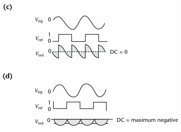
The simplest circuit is the half wave
averaging phase sensitive detector, in
which a simple field effect transistor
switch is driven by the reference
waveform and switches the signal into a
resistor capacitor filter (Fig. 11). An
inverting amplifier may be added to
producea full wave averaging, phase
sensitive detector. The phase sensitive
detector provides bipolar switching and
yields lower ripple, allowing less filtering
and therefore greater bandwidth (Fig. 12).
A single-diode phase sensitive detector
can be used for sine wave demodulation
as well (Fig. 13).
 
Legenda:
DC = averaged voltage of direct current component of waveform
Vout = output signal amplitude
Vref = reference signal amplitude
Vsig = test signal amplitude
Ficure 11. Half wave averaging, two-quadrant, phase
sensitive detector: (a) circuit diagram (Vier = 1
when switch
closed; V,e¢ = 0
when switch open); (b) Vsig in phase with Vie;
(©) sig 90 degrees out of phase with Vie (d) Vsig
180 degrees out of phase with Ver. Shading indicates part of
signal that is being averaged.
Legenda:
DC = averaged voltage of direct current component of waveform
Vout = output signal amplitude
Vref = reference signal amplitude
Vsig = test signal amplitude
Ficure 12. Full wave averaging phase sensitive detector:
(a) circuit diagram; (b) Vig in phase with Vier;
(©) Vsig 90 degrees out of phase with Vier (d) Vsig
180 degrees out of phase with Vref.
 
Legenda:
DC = averaged voltage of direct current component of waveform
R1, R2 = resistors
Vour = Output signal amplitude
Vref = reference signal amplitude
Vsig = test signal amplitude
Ficure 13. Single-diode phase sensitive detector: (a) circuit
diagram; (b) Vig in phase with Vier; (C) Vsig 90 degrees out of
phase with Vie; (d) Vsig 180 degrees out of phase with Vie.
A sampling phase sensitive detector
takes samples of the test waveform at two
points separated by 90 degrees and
usually digitizes these points directly
(Fig. 14). This approach allowsa fast
system response but requires a very clean
signal because the detector is very
sensitive to whatever noise is present at
the instant of sampling and has no
postdemodulator filtering. Pulsed eddy
current instruments may use this
technique to sample at a specific time
delay to obtain response relating to a
particular frequency.
 
Legenda:
DC = averaged voltage of direct current component of waveform
Vout = output signal amplitude
Vref = reference signal amplitude
Vsig = test signal amplitude
Vsw = sampled waveform amplitude
Ficure 14. Sampling phase sensitive detector: (a) circuit
diagram; (b) Vig in phase with Vier; (C) Vsig
90 degrees out of
ig
phase with Vier.
The four-quadrant multiplier is the
most accurate demodulator (Fig. 15). It
has no diode drops or switch artifacts to
cause nonlinearity. In a four-quadrant
multiplier, both the reference and the
signal inputs may swing in both positive
and negative directions. This flexibility is
in contrast to the operation of a
two-quadrant multiplier (Fig. 11).
 
Legenda
DC = averaged voltage of direct current component of waveform
Vout = output signal amplitude
Vref = reference signal amplitude
Vsig = test signal amplitude
Ficure 15. Analog multiplier, four-quadrant, phase sensitive
detector: (a) circuit diagram; (b) Vsig in phase with Vier;
(©) Vsig 90 degrees out of phase with Vier (d) Vsig
180 degrees out of phase with Vier
Integrated circuit multipliers with low
noise and high linearity are available off
the shelf from manufacturers. Even so, the
multiplier is usually the noise bottleneck
of the system. It has a characteristic noise
level and a limited input range, so it is
desirable to maximize the use of that
input range for optimal signal-to-noise
performance.
The reference signals used for
demodulation may be either sine waves or
square waves. The square waves are easily
generated from logical timing signals and
require little hardware to produce a clean
and accurate reference. The signal can be
expanded ina series of odd harmonic
terms:

where n is the nth frequency term, V is
the amplitude (volt) of the signal at any
time t (second), V,, is the maximum or
peak amplitude (volt) and @p is 2x times
the fundamental frequency (hertz).
This results in demodulation of the
odd multiples of the carrier frequency as
well. In a frequency domain multiplexed
system, this would prevent the instrument
from running frequencies that are odd
multiples of one another. In any system,
this restriction makes the test susceptible
to noise occurring at those frequencies.
For example, a 300 kHz test being
performed on a steam generator may be
contaminated by 900 kHz noise from a
nearby motor drive that is actually
switching at 100 kHz but generating an
odd harmonic that coincides with one
being demodulated in the eddy current
instrument.
The purest means of demodulation
then is to put a sine wave reference signal
into a high quality multiplier. This
demodulation requires extra hardware to
generate a second reference sine wave at
90 degrees out of phase from the driving
waveform. When these two reference
signals are clean and free of harmonic
distortion, the in-phase and out-of-phase
points will be the truest representation of
the end points of the phasor that
represents the test signal.
Note that an eddy current transducer
acts as a bandpass filter, filtering out noise
that may be present on the driving signal
and yielding a signal actually cleaner than
the reference signal. If this reference
signal is used for demodulation, the noise
is put right back into the signal.
Therefore, attention must be taken to
properly filter the sine wave references in
order to minimize noise. It is easier and
requires much less hardware to generate a
very low noise square wave for
demodulation than it is to produce a sine
wave of similar noise level in a digital
system, especially when that system is
required to operate over a broad
frequency range.
Time domain multiplexed instruments
require a single set of demodulators for
each transducer input. The reference
waveforms are multiplexed synchronously
with the test signal and the individual
frequencies are demodulated ina serial
fashion. Frequency domain multiplexed
instruments require a set of demodulators
operating at each frequency for each
transducer input. The synchronous
demodulator acts as a bandpass filter
centered on the carrier frequency. The
postdemodulator filter on each channel
must be narrow enough to reject the
other test frequencies. Time domain
multiplexed instruments typically have
much greater flexibility with frequency
selection because the filters are not
required to reject the other frequencies.
After the signal has been demodulated,
the system presents a useful
representation of the condition of the test
object. At this point, the results can be
analyzed by many means. The signal may
be directed to an analog meter or bar
graph for display or it may be digitized for
further manipulation and analysis.
Simple instruments used for
accept/reject testing of easily
distinguishable components on a
manufacturing line need only a
rudimentary display and will have a
comparator that analyzes the signal to
determine if it exceeds a set limit. The
only controls on such an instrument are
frequency, gain, phase and alarm level.
The frequency is determined by the
application. The gain is set to get an
adequate signal, the phase is rotated so
that the parameter of interest is
maximized on the display, the alarm level
is set and the instrument is ready. The
alarm may be audible or visible for
indication to a technician or it could
activate a sorting gate or a marking or
cutting device.
Analog instruments requiring two or
more parameters in analysis may use the
in-phase and out-of-phase signals as
horizontal and vertical components for
display on a cathode ray tube.
These analog instruments are limited
in bandwidth only by the operating
frequency, the number of frequencies used
and the bandwidth of the filters. They can
be constructed to perform extremely fast
testing. For example, there are
instruments with up to 60 kHz bandwidth
for use in bar, tube and wire applications
at part speeds up to 150 m-s"!
(29 500 ft-min-).
Digital instruments use an
analog-to-digital converter to digitize the
in-phase and out-of-phase components for
analysis and display. Time domain
multiplexed instruments use a pair of
analog-to-digital converters for each input
and digitize the signal from each
frequency sequentially. Frequency domain
multiplexed instruments may have a pair
of analog-to-digital converters sampling
simultaneously for each input or they
may have simultaneous sample-and-hold
circuits that are then sequentially
switched into a pair of analog-to-digital
converters.
The resolution and range of the
analog-to-digital converters is critical.
Generally, converters with a larger
number of bits have better signal-to-noise
performance. The greater the number of
bits, the greater the resolution, so a
converter must be selected for the
resolution desired for the application.
With a +10 V input, an eight-bit
analog-to-digital converter has 78 mV per
bit resolution, a 12-bit analog-to-digital
converter has about 5 mV resolution and
a 16-bit analog-to-digital converter has
305 pV resolution. To take advantage of
16 bits of resolution, the instrument noise
must be less than 1 mV.
Analog-to-digital converters have an
inherent noise floor and a limited input
range, so null and gain circuitry is often
used before the analog-to-digital
conversion to maximize the dynamic
range of the signals being digitized.
Generally a digital-to-analog converter is
used to generate a signal subtracted from
the test signal to obtain a null value. The
transducer is normally placed on a known
good part or on a clean reference standard
and a software routine calculates the null
values required and writes them to the
digital-to-analog converter. A digitally
adjustable gain may then be applied to
the signal to maximize use of the
dynamic range of the analog-to-digital
converter.
4. SAÍDA
4.1 MOSTRADOR
The displays of analog instruments are
relatively simple, enabling the user to
view and perform simple manipulations
of raw data. Generally, controls for phase,
gain, alarm levels and some filtering are
available. Analog recording of data via
magnetic tape and strip chart recorders
was common in the twentieth century but
has largely been replaced by digital data
storage. Analog instruments are used in a
few niche applications.
Digital data are generally displayed in a
complex plane presentation with
supporting strip chart and C-scan displays
as required by the application. The point
described by the in-phase and
out-of-phase components of the signal is
displayed as a flying dot and the digital
capabilities of the instrument allow
variable persistence, centering of the dot,
rotation of the signal and scaling of the
display. Digital systems allow setup of
calibration curves constructed from stored
data and automated analysis of signals as
compared to these curves.
Digital conductivity meters, calibrated
from conductivity reference standards,
feed subsequently acquired data into
algorithms that calculate conductivity and
distance of the conductivity probe from
the material surface for display in a
numerical format.
4.1.1 FILTRAGEM (R02)
Digital systems allow considerable
filtering capability. The primary use for
filtering of demodulated signals is to
separate desired from undesired signals
generated by the eddy current test. For
instance, if the signal contains a low
frequency component from probe motion
and a high frequency component from a
crack to be detected, then a high pass
filter could be used to attenuate the low
frequency component from the probe
motion while still passing the high
frequency component from the crack.
Time differentiation or high pass
filtering of test signals can be used if the
change in the state of the eddy current
signal conveys useful information but the
steady state output has no useful
information or masks the effect of the
useful information. An example of this is
the detection of cracks in wire or tubing
with a through-coil transducer. The steady
state signal does not convey useful
information. The signal will be generated
by motion of the wire laterally within the
coil or by the drift of the test system.
These effects would interfere with the
system’s ability to detect discontinuities of
a dynamic, time changing nature due to
the constant motion of the wire through
the coil. By differentiating the signal from
the demodulator, the effects of drift and
lateral motion will be rejected whereas the
discontinuity signals will still be seen.
Time integration of test signals can also
be used to minimize undesired
information. When unwanted noise is
present, it will often have a random and
widely spread frequency distribution
whereas the desired signal will not. If a
proper integration time constant is
selected, random noise can often be
reduced whereas the desired signal is left
relatively unchanged.
Time domain differentiation and
integration can also be interpreted in the
frequency domain. Differentiation
removes direct current components and
enhances high frequency components. It
acts as a high pass or low cut filter.
Conversely, a time integrator accentuates
direct current components and tends to
suppress high frequency components. It
acts as a low pass or high cut filter.
These filters can be combined with the
proper selection of cutoff frequencies
(time constants) both to remove low
frequency components from drift and to
suppress higher frequency random noise.
This composite filter is essentially a
bandpass filter.
4.1.2 RECONHECIMENTO DE SINAIS
Digital mixing, the combination of
components from different test
frequencies, allows the suppression of
unwanted parameters or signals from
structures such as support plates in tubing
applications while retaining the signature
of discontinuities beneath those
structures.
The combination of filtering, mixing
and signal recognition can be combined
with decision making algorithms to
produce powerful automated analysis
systems used in some applications
Alarms can be constructed digitally as
amplitude levels, boxes, ellipses or
whatever shape can be digitally described
for rejection or acceptance of parts.
Alarms from various frequencies or
transducers can be tagged and or or to
allow discrimination of different test
object conditions.
4.1.3 CONTROLE
Eddy current instruments are often used
as a component ina test system or
material handling system and so require
input and output capability to interface
with the controllers.
In the nuclear industry, robotic
manipulators are used to position and
manipulate the probes. The instruments
are part of an ethernet network, which
consists of data acquisition stations, data
analysis stations, data management
stations and control systems, some of
which may be thousands of kilometers
away. The instrument itself essentially
feeds data into this system for analysis
and control of the job.
In the manufacturing industry, an eddy
current instrument may communicate
with a programmable logic controller that
runs a material handling station or the
instrument may be required to perform
material control functions itself. These
instruments must have application
specific input and output capability to
provide the communications that can
perform the required control in a
demanding industrial environment.
demanding industrial environment.
Instruments are basically required to
trigger an alarm on certain conditions and
provide an output to mark, cut or reject a
part. Accept and reject information may
be digitally stored by an instrument or
accessed over a network for process
control.
Autores:
- James E. Cox, Zetec, Incorporated, Issaquah, Washington
- David J. Brown, Zetec, Incorporated, Issaquah, Washingtom
- Eric J. Strauts, TEEM Electronics, Park Ridge, Illinois
Referências
- Libby, H.L. Introduction to
Electromagnetic Nondestructive Test
Methods. New York, NY: John Wiley
and Sons (1971).
- Strauts, EJ. Section 11, “Electronic
Analysis Circuits for Eddy Current
Tests.” Nondestructive Testing Handbook,
second edition: Vol. 4, Electromagnetic
Testing. Columbus, OH: American
Society for Nondestructive Testing
(1986): p 265-314McMaster, R.C. “The Origins of
Electromagnetic Testing.” Materials
Evaluation. Vol. 43, No. 8. Columbus,
OH: American Society for
Nondestructive Testing (July 1986):
p 946-956.
|